CS-466/566: Math for AI

Module 05: Singular Value Decomposition

Dr. Mahmoud Mahmoud

The University of Alabama

2026-03-23

1. Eigen Decomposition for Dimensionality Reduction●

2. From Eigen to SVD (Why we need a new tool)○

3. Application: Image Compression○

4. SVD: Implementation○

5. Application: Principal Component Analysis (PCA)○

Eigen Decomposition: The “Sum of Patterns” View

General diagonalization: \(A = C D C^{-1}\).

For symmetric \(A\): eigenvectors are

orthonormal (\(C^{-1} = C^T\)), so \(A = C D C^T\).

Matrix Multiplication \(\rightarrow\) Sum of Rank-1 Matrices: \[ A = \underbrace{\begin{bmatrix} | & & | \\ v_1 & \dots & v_n \\ | & & | \end{bmatrix}}_{V} \underbrace{\begin{bmatrix} \lambda_1 & & \\ & \ddots & \\ & & \lambda_n \end{bmatrix}}_{\Lambda} \underbrace{\begin{bmatrix} - v_1^T - \\ \vdots \\ - v_n^T - \end{bmatrix}}_{V^T} = \sum_{i=1}^n \underbrace{\lambda_i}_{\text{scalar}} \cdot \underbrace{\mathbf{v}_i}_{n \times 1} \cdot \underbrace{\mathbf{v}_i^T}_{1 \times n} \]

Insight: Each term \(\lambda_i \mathbf{v}_i \mathbf{v}_i^T\) is an \(n \times n\) matrix. If \(\lambda_i \approx 0\), that term vanishes \(\rightarrow\) Sparsity / Dimensionality Reduction!

1. Eigen Decomposition for Dimensionality Reduction✓

2. From Eigen to SVD (Why we need a new tool)●

3. Application: Image Compression○

4. SVD: Implementation○

5. Application: Principal Component Analysis (PCA)○

Eigen Vectors for Square Matrices Requirement

Let’s consider a non-square matrix \(A\): \[ A \mathbf{x} = \begin{bmatrix} 1 & 0 \\ 0 & 1 \\ 0 & 0 \end{bmatrix}_{(3 \times 2)} \begin{bmatrix} x_1 \\ x_2 \end{bmatrix}_{(2 \times 1)} \]

if \(x \in \mathbb{R}^2\) then \(Ax \in \mathbb{R}^3\)

So it can never equal \(\lambda x \in \mathbb{R}^2\).

Eigen decomposition only works for square matrices!

Why Eigen Decomposition is Not Always Possible

Eigen decomposition / diagonalization assumes:

\(A\) is square (\(n \times n\))
and has enough linearly independent eigenvectors

But ML data is usually rectangular

\(X\) = (number of samples) \(\times\) (number of features)
e.g., \(X \in \mathbb{R}^{10000 \times 768}\)

So… How to find a similar concept to eigenvectors for a non-square matrix?

This is exactly why we use SVD.

Trick: Build Two Square Matrices from Any \(A\)

Let \(A\) be any \(m \times n\) matrix (maybe not square).

We can always form: \[ AA^T \in \mathbb{R}^{m \times m}, \quad A^TA \in \mathbb{R}^{n \times n} \] Both are:

square
symmetric
eigenvalues are \(\ge 0\)

So even if \(A\) is rectangular, \(AA^T\) and \(A^TA\) have real eigenvectors.

Why is \(AA^T\) Symmetric and Square?

Square: If \(A\) is \(m \times n\), then \(A^T\) is \(n \times m\). \[ \underbrace{A}_{m \times n} \cdot \underbrace{A^T}_{n \times m} = \underbrace{AA^T}_{m \times m} \]

\[ \underbrace{\begin{bmatrix} 1 & 2 \\ 3 & 4 \\ 5 & 6 \end{bmatrix}}_{3 \times 2} \cdot \underbrace{\begin{bmatrix} 1 & 3 & 5 \\ 2 & 4 & 6 \end{bmatrix}}_{2 \times 3} = \underbrace{\begin{bmatrix} 5 & 11 & 17 \\ 11 & 25 & 39 \\ 17 & 39 & 61 \end{bmatrix}}_{3 \times 3} \]

SVD Roadmap

Our Goal: Factor any \(m \times n\) matrix \(A\) into \(A = U \Sigma V^T\).

The 3-Step Journey:

Find \(V\)?
Find \(\Sigma\) (Singular values)?
Find \(U\)?

Since \(A^TA\) is symmetric → we can always find orthogonal eigenvectors in an indirect way!

SVD Derivation (Part 1)

Step 1: Start with \(A^TA\)

We can always find the eigenvalues and eigenvectors of \(A^TA\) (even if \(A\) is not square): \[ \underbrace{A^TA}_{n \times n} \underbrace{\mathbf{v}_i}_{\substack{\text{right eigenvectors} \\ n \times 1}} = \lambda_i \underbrace{\mathbf{v}_i}_{\substack{\text{right eigenvectors} \\ n \times 1}} \] These \(\mathbf{v}_i\) are our Right Singular Vectors.

Step 2: Define Singular Values

Since \(\lambda_i \ge 0\): \(\quad \sigma_i = \sqrt{\lambda_i}\)

\[ \underbrace{A^TA}_{n \times n} \underbrace{\mathbf{v}_i}_{\substack{\text{right eigenvectors} \\ n \times 1}} = \sigma_i^2 \underbrace{\mathbf{v}_i}_{\substack{\text{right eigenvectors} \\ n \times 1}} \]

SVD Derivation (Part 2)

Step 3: Multiply both sides by \(A\): \[ \underbrace{(AA^T)}_{m \times m}\underbrace{(A\mathbf{v}_i)}_{\substack{\text{eigenvector!} \\ m \times 1}} = \sigma_i^2 \underbrace{(A\mathbf{v}_i)}_{\substack{\text{eigenvector!} \\ m \times 1}} \]

So \(A\mathbf{v}_i\) is an eigenvector of \(AA^T\)!

Define: \(\mathbf{u}_i = \frac{A\mathbf{v}_i}{\sigma_i}\) (normalized).

Then: \(A \mathbf{v}_i = \sigma_i \mathbf{u}_i\) ← core SVD relation!

Step 4: Stack & Finish

Stack vectors: \(\underbrace{V}_{n \times n} = [\mathbf{v}_1, \dots, \mathbf{v}_n], \quad \underbrace{U}_{m \times m} = [\mathbf{u}_1, \dots, \mathbf{u}_m]\)

The key relation: \(A\mathbf{v}_i = \sigma_i \mathbf{u}_i \implies AV = U\Sigma \implies\) \(A = U \Sigma V^T\) ✅

The One Relationship to Remember

SVD gives paired vectors \((u_i, v_i)\) such that: \[ \underbrace{A}_{m \times n} \cdot \quad \underbrace{v_i}_{n \times 1} \quad = \quad \sigma_i \quad \underbrace{u_i}_{m \times 1} \] Meaning:

\(v_i\): a special input direction
\(A v_i\): lands exactly on direction \(u_i\)
scaled by \(\sigma_i\)

So \(A\) maps one special axis to another special axis, with a known scale.

Numeric Example (1/8)

\[ A = \begin{bmatrix} 3 & 2 & 2 \\ 2 & 3 & -2 \end{bmatrix}_{2 \times 3} \quad \implies \quad A^T = \begin{bmatrix} 3 & 2 \\ 2 & 3 \\ 2 & -2 \end{bmatrix}_{3 \times 2} \]

Step 1: Compute \(A^T A\): \[ A^T A = \begin{bmatrix} 3 & 2 \\ 2 & 3 \\ 2 & -2 \end{bmatrix}_{3 \times 2} \begin{bmatrix} 3 & 2 & 2 \\ 2 & 3 & -2 \end{bmatrix}_{2 \times 3} = \begin{bmatrix} 13 & 12 & 2 \\ 12 & 13 & -2 \\ 2 & -2 & 8 \end{bmatrix}_{3 \times 3} \]

Numeric Example (2/8)

Step 2: Eigenvalues of \(A^T A\) — solve \(\det(A^T A - \lambda I) = 0\): \[ \det\left( \begin{bmatrix} 13 - \lambda & 12 & 2 \\ 12 & 13 - \lambda & -2 \\ 2 & -2 & 8 - \lambda \end{bmatrix} \right) = 0 \]

Cofactor expansion along row 1: \[ = (13-\lambda) \det\begin{bmatrix} 13-\lambda & -2 \\ -2 & 8-\lambda \end{bmatrix} - 12 \det\begin{bmatrix} 12 & -2 \\ 2 & 8-\lambda \end{bmatrix} + 2 \det\begin{bmatrix} 12 & 13-\lambda \\ 2 & -2 \end{bmatrix} \]

Compute each 2×2 determinant: \[ = (13-\lambda)[(13-\lambda)(8-\lambda) - 4] - 12[12(8-\lambda) + 4] + 2[-24 - 2(13-\lambda)] \]

\[ = \lambda^3 - 34\lambda^2 + 225\lambda = \lambda(\lambda - 25)(\lambda - 9) = 0 \] \(\implies \lambda_1 = 25, \quad \lambda_2 = 9, \quad \lambda_3 = 0\)

Numeric Example (3/8)

Step 3: Singular Values (\(\sigma = \sqrt{\lambda}\)): \[ \sigma_1 = \sqrt{25} = 5, \quad \sigma_2 = \sqrt{9} = 3, \quad \sigma_3 = \sqrt{0} = 0 \]

The non-zero singular values are \(\sigma_1 = 5\) and \(\sigma_2 = 3\).

Since \(A\) is \(2 \times 3\), we have at most 2 non-zero singular values.

Numeric Example (4/8): Find \(V\) (Part a)

Step 4: Find eigenvectors of \(A^TA\) for each \(\lambda\)

For \(\lambda_1 = 25\): solve \((A^TA - 25I)\mathbf{v}_1 = 0\) \[ \begin{bmatrix} 13-25 & 12 & 2 \\ 12 & 13-25 & -2 \\ 2 & -2 & 8-25 \end{bmatrix} \mathbf{v}_1 = \begin{bmatrix} -12 & 12 & 2 \\ 12 & -12 & -2 \\ 2 & -2 & -17 \end{bmatrix} \mathbf{v}_1 = \mathbf{0} \]

Row reduce → from row 1: \(-12v_1 + 12v_2 + 2v_3 = 0 \implies v_1 = v_2 + \frac{v_3}{6}\)

Setting \(v_3 = 0, v_2 = 1 \implies v_1 = 1\). Normalize: \[ \mathbf{v}_1 = \frac{1}{\sqrt{2}}\begin{bmatrix} 1 \\ 1 \\ 0 \end{bmatrix} \]

Numeric Example (5/8): Find \(V\) (Part b)

For \(\lambda_2 = 9\): solve \((A^TA - 9I)\mathbf{v}_2 = 0\) \[ \begin{bmatrix} 13-9 & 12 & 2 \\ 12 & 13-9 & -2 \\ 2 & -2 & 8-9 \end{bmatrix} \mathbf{v}_2 = \begin{bmatrix} 4 & 12 & 2 \\ 12 & 4 & -2 \\ 2 & -2 & -1 \end{bmatrix} \mathbf{v}_2 = \mathbf{0} \]

Row reduce → solution: \(v_1 = 1, v_2 = -1, v_3 = 4\) (proportional). Normalize: \[ \mathbf{v}_2 = \frac{1}{\sqrt{18}}\begin{bmatrix} 1 \\ -1 \\ 4 \end{bmatrix} \]

Numeric Example (6/8): Find \(V\) (Part c)

For \(\lambda_3 = 0\): solve \((A^TA - 0I)\mathbf{v}_3 = 0\) \[ \begin{bmatrix} 13 & 12 & 2 \\ 12 & 13 & -2 \\ 2 & -2 & 8 \end{bmatrix} \mathbf{v}_3 = \mathbf{0} \]

Row reduce → solution: \(v_1 = -2, v_2 = 2, v_3 = 1\) (proportional).

Normalize: \[ \mathbf{v}_3 = \frac{1}{3}\begin{bmatrix} -2 \\ 2 \\ 1 \end{bmatrix} \]

Numeric Example (7/8): Find \(U\)

Step 5: Find \(U\) — use \(\mathbf{u}_i = \frac{A\mathbf{v}_i}{\sigma_i}\)

\(\mathbf{u}_1 = \frac{1}{\sigma_1} A \mathbf{v}_1 = \frac{1}{5} \begin{bmatrix} 3 & 2 & 2 \\ 2 & 3 & -2 \end{bmatrix} \cdot \frac{1}{\sqrt{2}}\begin{bmatrix} 1 \\ 1 \\ 0 \end{bmatrix} = \frac{1}{5\sqrt{2}} \begin{bmatrix} 5 \\ 5 \end{bmatrix} = \frac{1}{\sqrt{2}}\begin{bmatrix} 1 \\ 1 \end{bmatrix}\)

\(\mathbf{u}_2 = \frac{1}{\sigma_2} A \mathbf{v}_2 = \frac{1}{3} \begin{bmatrix} 3 & 2 & 2 \\ 2 & 3 & -2 \end{bmatrix} \cdot \frac{1}{\sqrt{18}}\begin{bmatrix} 1 \\ -1 \\ 4 \end{bmatrix} = \frac{1}{3\sqrt{18}} \begin{bmatrix} 9 \\ -9 \end{bmatrix} = \frac{1}{\sqrt{2}}\begin{bmatrix} 1 \\ -1 \end{bmatrix}\)

Numeric Example (8/8)

Step 6: Build \(\Sigma\): \[ \Sigma = \begin{bmatrix} 5 & 0 & 0 \\ 0 & 3 & 0 \end{bmatrix}_{2 \times 3} \]

Final Decomposition (\(A = U \Sigma V^T\)): \[ \underbrace{A}_{2 \times 3} = \underbrace{U}_{2 \times 2} \cdot \underbrace{\Sigma}_{2 \times 3} \cdot \underbrace{V^T}_{3 \times 3} \]

\[ \implies \begin{bmatrix} 3 & 2 & 2 \\ 2 & 3 & -2 \end{bmatrix} = \underbrace{\begin{bmatrix} \frac{1}{\sqrt{2}} & \frac{1}{\sqrt{2}} \\ \frac{1}{\sqrt{2}} & \frac{-1}{\sqrt{2}} \end{bmatrix}}_{U} \underbrace{\begin{bmatrix} 5 & 0 & 0 \\ 0 & 3 & 0 \end{bmatrix}}_{\Sigma} \underbrace{\begin{bmatrix} \frac{1}{\sqrt{2}} & \frac{1}{\sqrt{2}} & 0 \\ \frac{1}{\sqrt{18}} & \frac{-1}{\sqrt{18}} & \frac{4}{\sqrt{18}} \\ \frac{-2}{3} & \frac{2}{3} & \frac{1}{3} \end{bmatrix}}_{V^T} \]

1. Eigen Decomposition for Dimensionality Reduction✓

2. From Eigen to SVD (Why we need a new tool)✓

3. Application: Image Compression●

4. SVD: Implementation○

5. Application: Principal Component Analysis (PCA)○

The Best Low-Rank Approximation

SVD allows us to represent an image (matrix \(A\)) as a sum of rank-1 patterns: \[ A = \sigma_1 u_1 v_1^T + \sigma_2 u_2 v_2^T + \cdots + \sigma_r u_r v_r^T \]

By keeping only the first \(k\) terms, we get the best possible approximation of rank \(k\).

Original

k=5

k=5 (Blurry)

k=20

k=20 (Better)

k=50

k=50 (Almost Perfect)

1. Eigen Decomposition for Dimensionality Reduction✓

2. From Eigen to SVD (Why we need a new tool)✓

3. Application: Image Compression✓

4. SVD: Implementation●

5. Application: Principal Component Analysis (PCA)○

SVD in NumPy

In Python, we use numpy.linalg.svd:

import numpy as np

#> Compute SVD
U, S, Vt = np.linalg.svd(A, full_matrices=False)

Key Details:

S is returned as a 1D array (vector), not a diagonal matrix.
Vt is already transposed (\(V^T\)).
full_matrices=False computes the Economy SVD (faster).

The singular values in \(S\) are returned sorted in descending order: \[ \sigma_1 \ge \sigma_2 \ge \sigma_3 \ge \dots \ge 0 \]

Reconstructing from SVD

To rebuild the matrix (or an approximation), we need to turn S back into a diagonal matrix:

#> Reconstruct A using all components
A_reconst = U @ np.diag(S) @ Vt

#> Approximation with top k components
k = 10
#> S[:k] is the first k elements, np.diag makes it k x k
A_k = U[:, :k] @ np.diag(S[:k]) @ Vt[:k, :]

Setting the value of \(k\) controls the rank of the approximation: \[ A_k = U \cdot \Sigma_k \cdot V^T \]

1. Eigen Decomposition for Dimensionality Reduction✓

2. From Eigen to SVD (Why we need a new tool)✓

3. Application: Image Compression✓

4. SVD: Implementation✓

5. Application: Principal Component Analysis (PCA)●

The Curse of Dimensionality

Real-world data has many features:

Student records: Height, Weight, GPA, SAT, …
Images: thousands of pixels
Text: thousands of word frequencies
Genomics: ~20,000 genes

As dimensions \(\uparrow\), data becomes sparse, distances become meaningless, and models overfit.

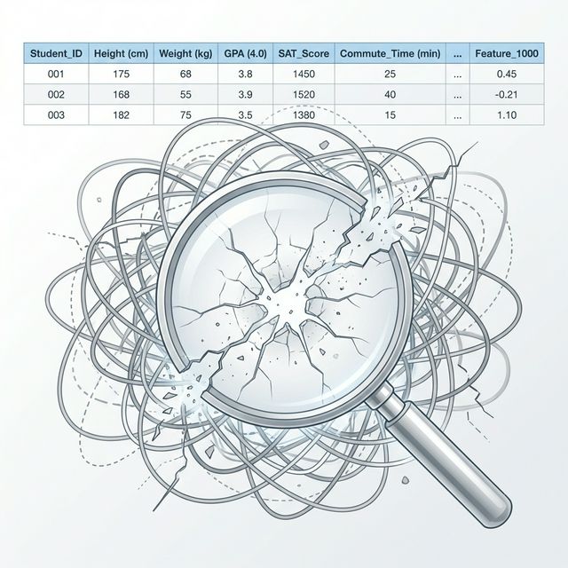
Question: Can we find a smaller set of variables that captures most of the information?

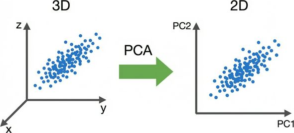
What Does PCA Do?

PCA finds a new coordinate system where:

Axes point along the directions of maximum variance
Axes are orthogonal to each other
We can drop axes with low variance → dimensionality reduction

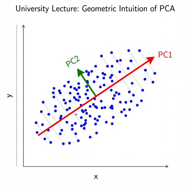
Geometric Intuition

Given a cloud of data points:

PC1 = direction of greatest spread (variance)
PC2 = direction of greatest spread perpendicular to PC1
PC3 = … and so on

Each Principal Component captures the next most important pattern in the data.

PCA finds the best linear summary of your data in fewer dimensions.

PCA Algorithm Summary

Step	Operation	Result
1	Center: \(\bar{X} = X - \mathbf{1}\boldsymbol{\mu}^T\)	Zero-mean data
2	SVD: \(\bar{X} = U \Sigma V^T\)	Get components
3	Choose \(k\) components	Keep top \(k\) columns of \(V\)
4	Project: \(Z = \bar{X} V_k\)	Reduced data (\(n \times k\))

Result: We go from \(d\) features → \(k\) features, where \(k \ll d\).

PCA in Python

Using SVD directly (NumPy):

import numpy as np

#> Center the data
X_centered = X - X.mean(axis=0)

#> SVD
U, S, Vt = np.linalg.svd(X_centered, full_matrices=False)

#> Project onto top k components
k = 2
X_reduced = X_centered @ Vt[:k, :].T   # n x k

Why Does SVD Give Us the Principal Components?

Step 1: Center the data

Given data matrix \(X\) (\(n\) samples \(\times\) \(d\) features), subtract the mean: \[ \bar{X} = X - \mathbf{1}\boldsymbol{\mu}^T \]

Step 2: The covariance matrix is \[ C = \frac{1}{n-1} \bar{X}^T \bar{X} \] Its eigenvectors = principal components, eigenvalues = variance along each PC.

Step 3: Apply SVD

\(\bar{X} = U \Sigma V^T \implies\) the columns of \(V\) are the principal components!

\[ C = \frac{1}{n-1} V \Sigma^2 V^T \]

How Many Components to Keep?

The variance explained by each component is:

\[ \text{Var explained by PC}_i = \frac{\sigma_i^2}{\sum_{j=1}^{d} \sigma_j^2} \]

Rule of thumb: keep enough components to explain 90-95% of total variance.

Example: If \(\sigma_1 = 10, \sigma_2 = 5, \sigma_3 = 1, \sigma_4 = 0.1\)

PC	\(\sigma_i^2\)	% Variance	Cumulative
1	100	79.4%	79.4%
2	25	19.8%	99.2%
3	1	0.8%	100.0%
4	0.01	~0%	100.0%

→ Keeping just 2 PCs captures 99.2% of the information!

Thank You!

CS-466/566: Math for AI

TABLE OF CONTENTS

Eigen Decomposition: The “Sum of Patterns” View

TABLE OF CONTENTS

Eigen Vectors for Square Matrices Requirement

Why Eigen Decomposition is Not Always Possible

Trick: Build Two Square Matrices from Any \(A\)

Why is \(AA^T\) Symmetric and Square?

SVD Roadmap

SVD Derivation (Part 1)

SVD Derivation (Part 2)

The One Relationship to Remember

Numeric Example (1/8)

Numeric Example (2/8)

Numeric Example (3/8)

Numeric Example (4/8): Find \(V\) (Part a)

Numeric Example (5/8): Find \(V\) (Part b)

Numeric Example (6/8): Find \(V\) (Part c)

Numeric Example (7/8): Find \(U\)

Numeric Example (8/8)

TABLE OF CONTENTS

The Best Low-Rank Approximation

TABLE OF CONTENTS

SVD in NumPy

Reconstructing from SVD

TABLE OF CONTENTS

The Curse of Dimensionality

What Does PCA Do?

Geometric Intuition

PCA Algorithm Summary

PCA in Python

Why Does SVD Give Us the Principal Components?

How Many Components to Keep?

Thank You!